Renderman Course: Fur in Stuart Little
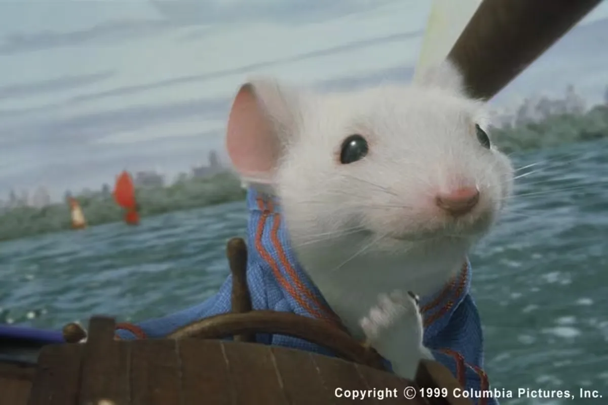
In 2000, I was invited to help teach a Siggraph session on Renderman. I was able to present the work of many people at Sony Imageworks who helped bring our furry hero to life. Stuart Little was the first CG character to lead in a live-action movie, and there were plenty of things to work out to make it possible. In addition to the fur detailed below, there was a lot of effort put into the simulation of his clothing and just about every other aspect of the character.
The show was led by Sr VFX Supervisor John Dykstra, and VFX Supervisor Jerome Chen. I learned a ton on this film and was very honored to get to present these notes in the SIGGRAPH Renderman course that year.
The majority of the development of the fur technology for Stuart Little was performed by Clint Hanson and Armin Bruderlin. I helped build this presentation and organize these notes. Sony Imageworks was supportive of our efforts to share our learnings with the computer graphics community for which I am very grateful.
{{% toc %}}
Written By: Rob Bredow
Abstract
Realistic fur instantiation and shading is a challenge that was undertaken during recent work on the film Stuart Little. This talk will detail some of the techniques used to create Stuart Little’s furry coat and how Renderman was used to light and shade the mouse’s hair.
Goals
- Must be cute (and realistic).
- Retain detailed looking fur regardless of size on screen
- Realistic lighting model
- Needs flexible controls for cases where realism is not desired
- Handle multiple lighting environments (day, night, sourcey, diffuse)
- wet/shiny/dirty
- Fur interaction with environment
- wind
- other objects
- self
- clothing
- Multiple furred characters on screen at one time
- Efficient enough for nearly 500 shots
Design Overview
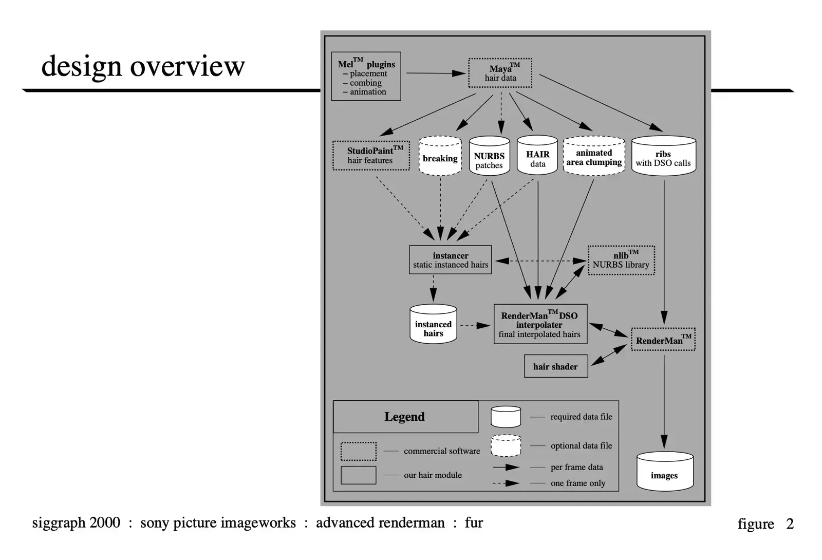
The general pipeline consists of two major processes, those that happen once for each character and those that happen once for each frame. The former consist of gathering all of the data which controls the look and contouring of the fur and calculating as much as possible to be stored in a series of data files. The second process consists of the actual creation of the fur on the character from these data files at the time of the render.
Most of the data for the first set of processes (to design the look of the hair) is managed through MEL scripts in Maya and attributes controlled through StudioPaint. The instancer is then run to compile all of the appropriate data files into a “instanced hair” data file which specifies the location of each hair on the character. This step only has to be calculated one time at the initial setup of the character or if there is a change to the fur data files.
It is important in the design of the system to leave as much of the large dataset creation until the latest possible point in the pipeline. So, the actual RiCurve primitives are not “grown” onto the surfaces until the time of the render when Renderman notices the DSO references built into the rib file and calls the interpolator DSO. The DSO then generates the rib data which contains an RiCurve for each hair contoured to the surface appropriately and taking into account the character’s animation. The hair is then shaded with a standard renderman shader and the output image is generated.
Fur Instantiation (the interpolator)
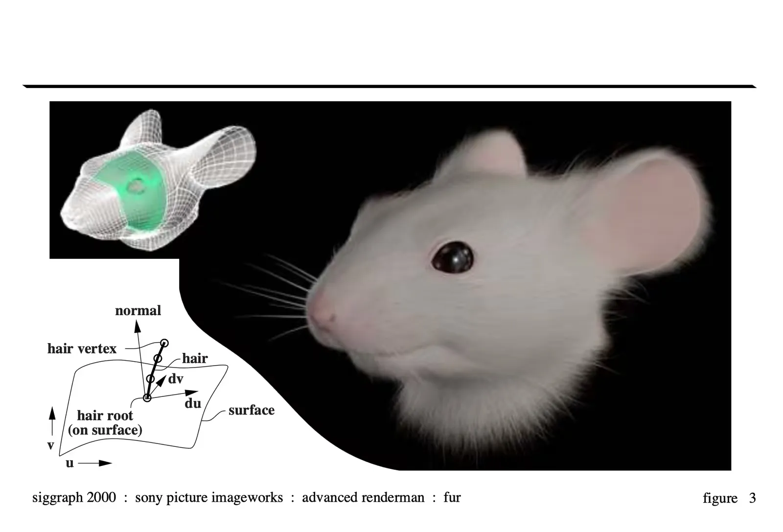
The interpolator performs the function of “growing” the RiCurve primitives from all of the input data.
instanced hair data The instancer specifies the position of each of the individual hairs for each patch in terms of the u, v coordinate of the surface. animated nurbs patches These patches form the skin of the character and are used to position the hair in the correct 3d space and orientation according to the surface normal, and the surface derivative information at the position of interest. hair data from Maya and optionally animated area clumping information. This data is used to generate the 4 point curve taking into account the combing information and the other fur attributes specified in the data files.
Clumping
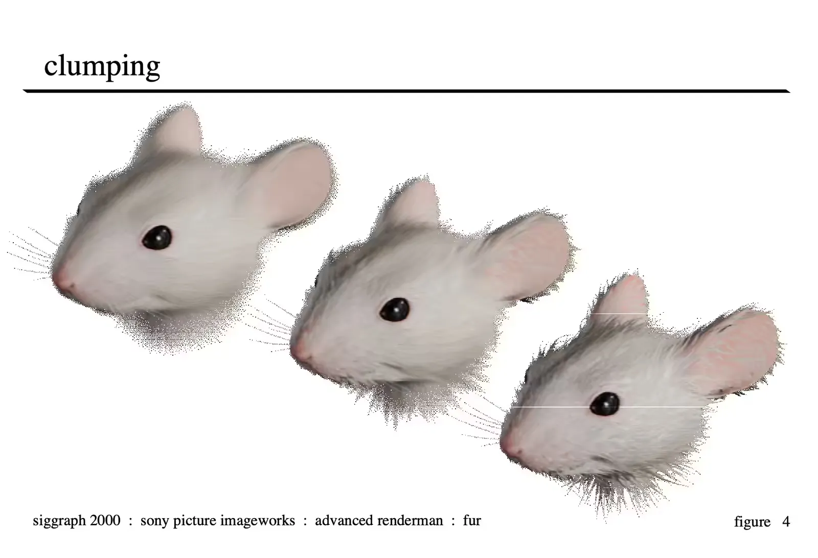
Clumping of hairs can occur when the fur gets wet due to the surface tension of water. The overall effect is that sets of neighboring hairs tend to join into a single point creating a kind of cone-shaped “super-hair” or circular clump. We have implemented two kinds of clumping techniques: static area clumping and animated area clumping. The former generates hair clumps in fixed predefined areas on the model, whereas the latter allows for the areas that are clumped to change over time. In both cases, we provide parameters which can be animated to achieve various degrees of dry-to-wet fur looks which can also be animated over time.
Static Area Clumping
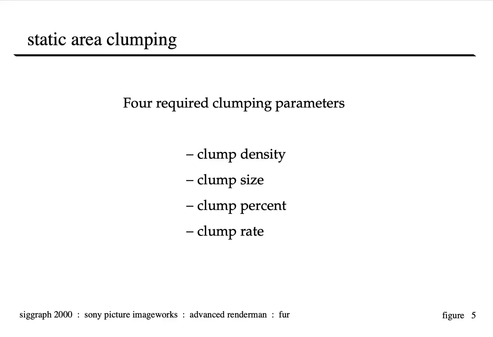
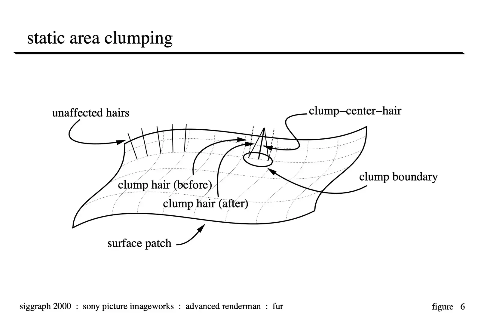
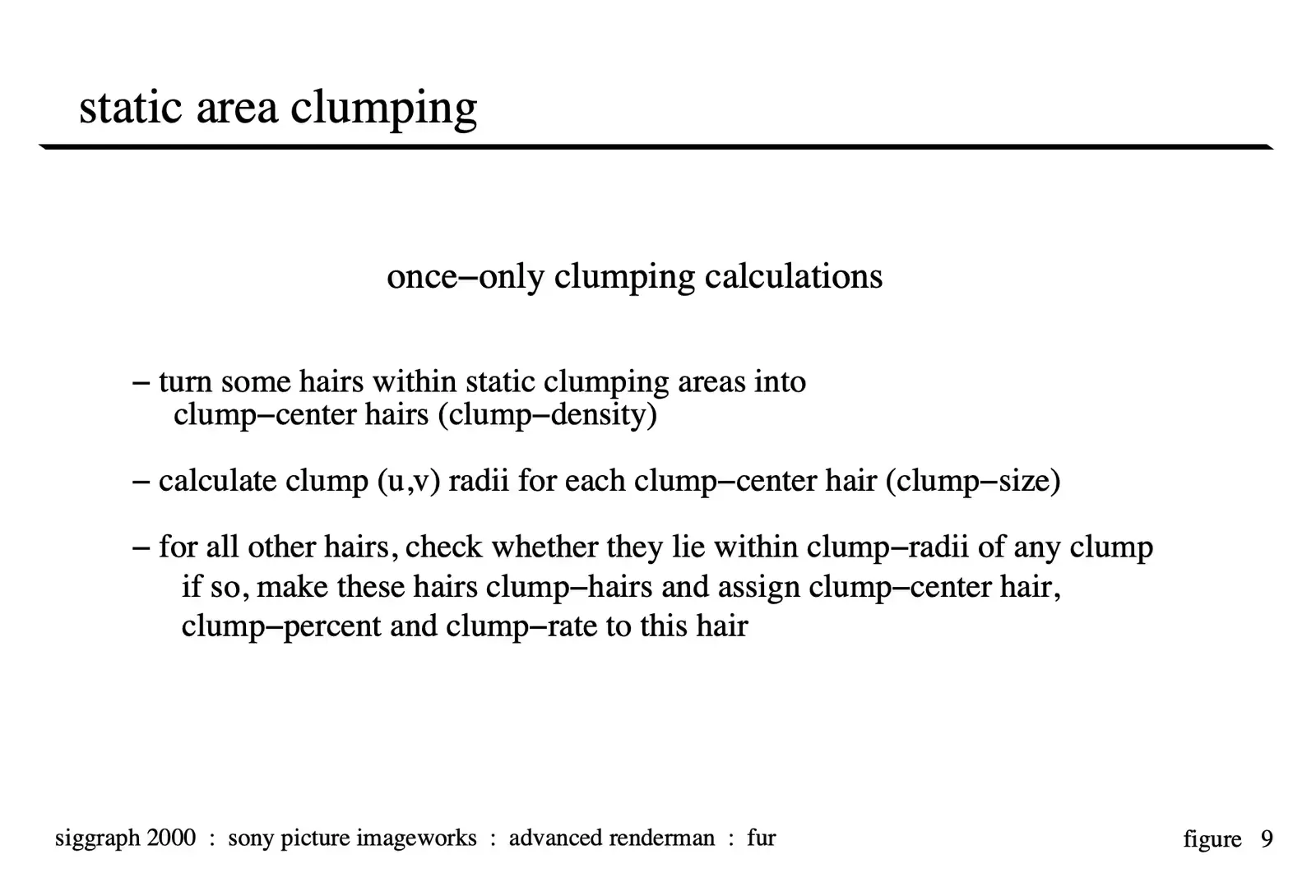
There are four required clumping input parameters: clump-density, clump-size, clump-percent and clump-rate. Clump-density specifies how many clumps should be generated per square area. Our clump method translates this density into an actual number of clumps, depending on the size of each surface patch. We call the center hair of each clump the clump-center hair, and all the other member hairs of that clump, which are attracted to this clump-center hair, clump hairs.
Clump-size defines the area of a clump in world space. To determine clump membership of each final hair, our clump method first converts the specified clump-size into a u-radius and v-radius component in parametric surface space at each clump-center hair location. It then checks for each hair, whether it falls within the radii of a clump-center hair; if so, that clump-center hair’s index is stored with the hair; if not, the hair is not part of any clump, i.e. is not a clump hair. Our clump method also has an optional clump-size noise parameter to produce random variations in the size of the clumps. Furthermore, texture maps for all four parameters can be created and specified by the user, one per surface patch, to provide local control: for instance, if clump-size maps are specified, the global clump-size input parameter is multiplied for a particular clump (clump center hair) at (u,v) on a surface patch with the corresponding normalized (s,t) value in the clump-size feature map for that surface patch. Also, a clump-area feature map can be provided to limit clumping to specified areas on surface patches rather than the whole model.
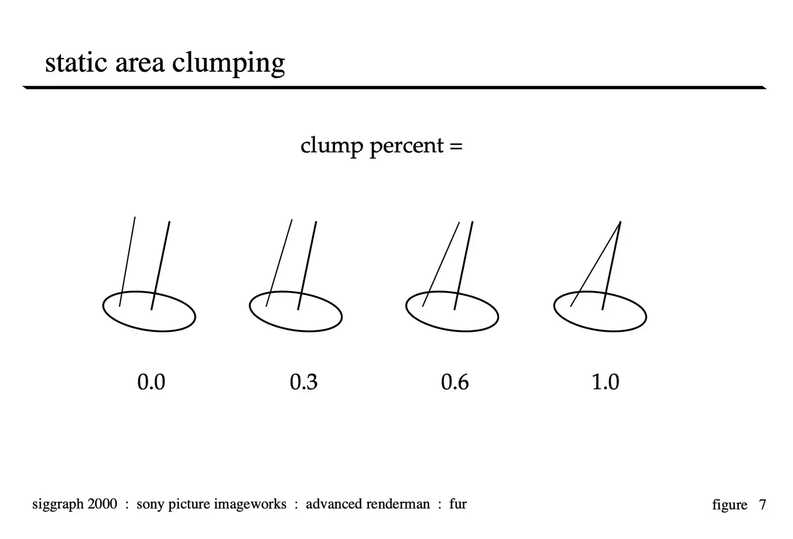
Clump-percent controls the amount the hair is drawn to the clump-center-hair. This is done in a linear fashion where the endpoint of the hair is effected 100% and the base of the hair (where it is connected to the patch) is never moved. Higher clump-percent values yield more wet looking fur.
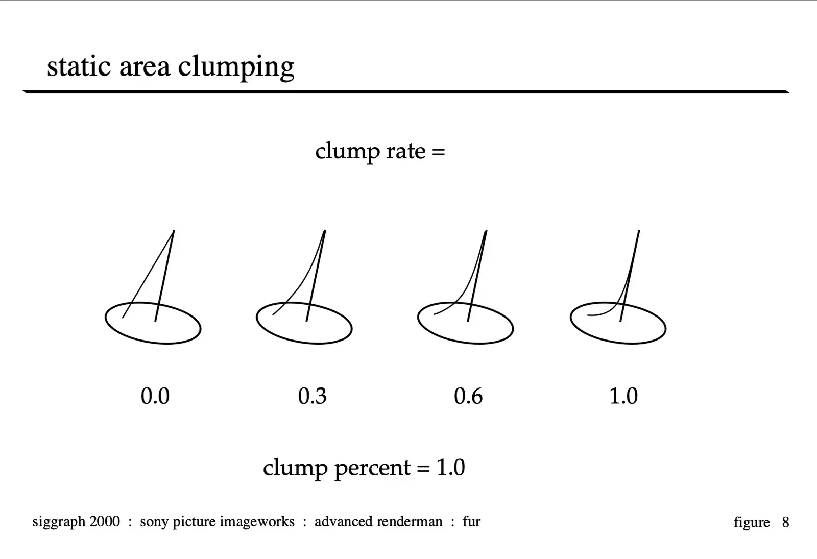
Clump-rate is the control used to dial in how much the fur is curved near the base to match the clump-center-hair. This is also interpolated over the length of the fur so the base of the fur is never effected by the clumping procedure. Dialing this parameter up yields dramatic increases in the wetness look of the character as the individual hairs are drawn more strongly to the clump centers.
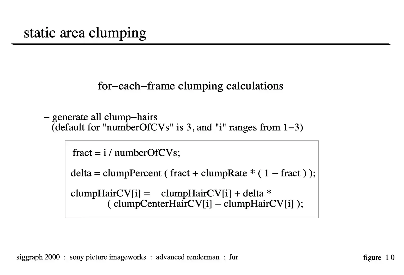
The equations for calculating the clumped vertices are illustrated above. The vertices of each clump hair (except the root vertex) are re-oriented towards their corresponding clump-center hair vertices from their dry, combed position, where the default value for numberOfCVs is 3 (4 minus the root vertex), and the index for the current control vertex, i, ranges from 1-3.
It is noted that both rate and percent operations change the lengths of clumps hairs. We have not, however, observed any visual artifacts even as these values are animated over the course of an animation.
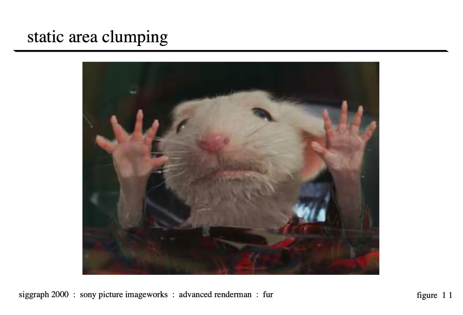 Image Copyright 2000 by Columbia Pictures Industries Inc., All Rights Reserved
Animated Area Clumping
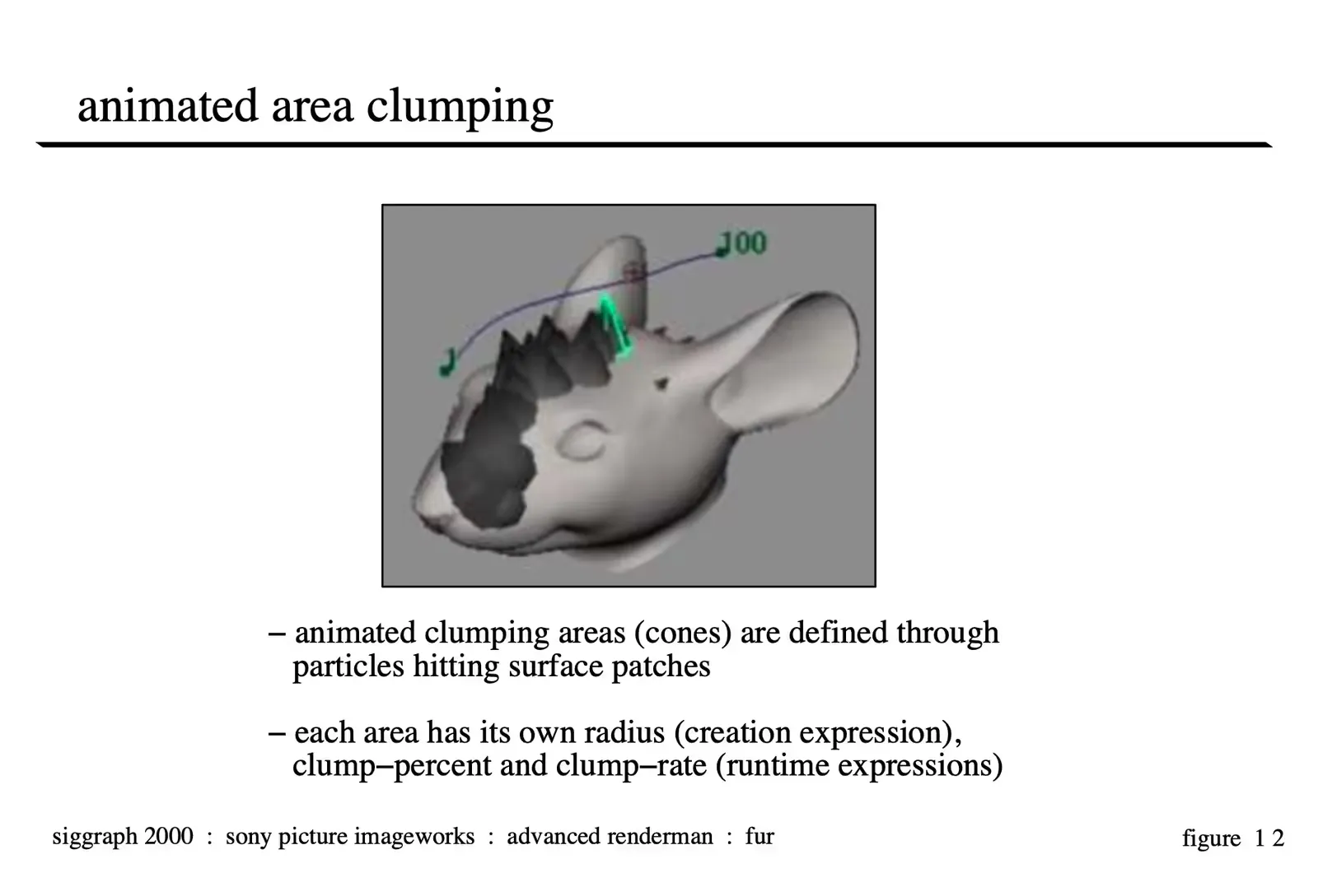
Animated area clumping is desirable if we want to simulate spouts of water or raindrops hitting the fur and making it increasingly wet. To simulate this, animated clumping areas are defined in an animation system through particles hitting surface patches. These particles originate from one or more emitters, whose attributes determine, for instance, the rate and spread of the particles. Once a particle hits a surface patch, a circular clumping area is created on the patch at that (u,v) location, with clump-percent, clump-rate and radius determined by a creation expression. Similar to static clump-size, this radius is converted into a corresponding u-radius and v-radius. Runtime expressions then define clump percent and rate, to determine how quickly and how much the fur “gets” wet. The above image shows a snapshot of animated clumping areas, where each area is visualized as a cone (the most recent cone is highlighted). In this case, one particle emitter is used and has been animated to follow the curve above the head.
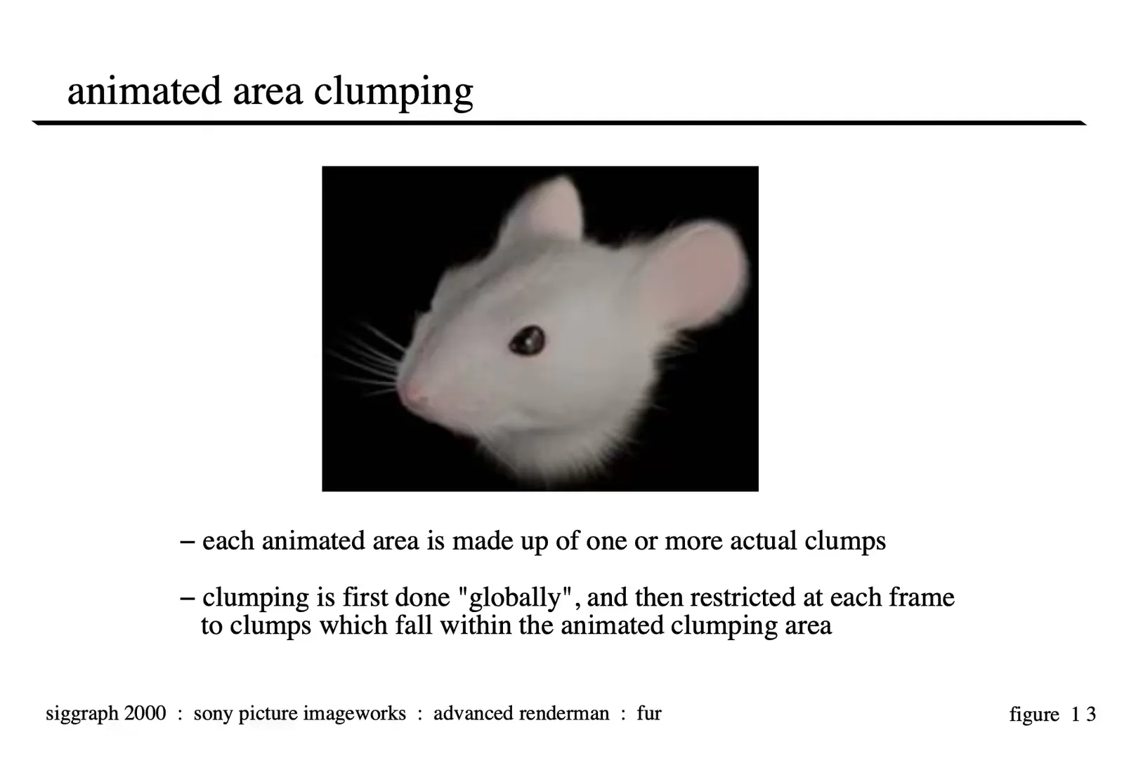
Once the animated clumping areas are defined for each frame of an animation, hairs which fall within these clumping areas are clumped. Clumping areas are usually much bigger than a clump, thus containing several individual clumps. In our implementation, we first apply static area clumping to the whole model as described above, and then restrict the clumping procedure to hairs within the animated clumping areas at each frame (i.e. to clumps which fall within any clumping area), so that final hairs of clumps outside clumping areas are normally produced as “dry” hairs. To determine whether a clump falls within a clumping area, the clump method checks at each frame whether the (u,v) distance between the clump-center hair of the clump and the center of the clumping area is within the (u,v) radii of the clumping area. For clumps in overlapping clumping areas, the values for clump-percent and rate are added to generate wetter fur. The above image shows the resulting clumped hairs in the areas defined in the previous image

One problem with animated clumping areas has not been addressed yet: they can straddle surface patch boundaries as shown in this illustration, which shows a top view of a clumping area (grey-colored cone): the center of this clumping area (black dot) is on patch P1, but the area straddles onto patch P2 and P3 (across a T-junction; seams are drawn as bold lines). Since our clumping areas are associated with the surface which contains the center of the clumping area, i.e. the position where the particle hit, portions of a clumping area straddling neighboring patches are ignored. This would lead to discontinuities in clumping of the final fur.
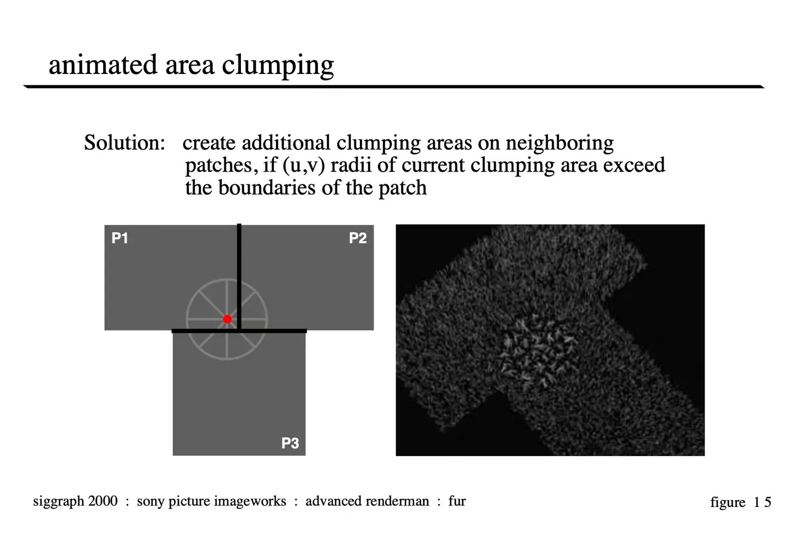
The solution presented here utilizes our surface seam and topology generator module: whenever a new particle hits a surface, the clump method checks at each frame whether the (u,v) radii exceed the boundaries of that surface; if so, it calculates the (u,v) center and new (u,v) radii of this clumping area with respect to the affected neighboring patches. These “secondary” clumping areas on affected neighboring patches are then included in the calculations above to determine which clumps fall into clumping areas.
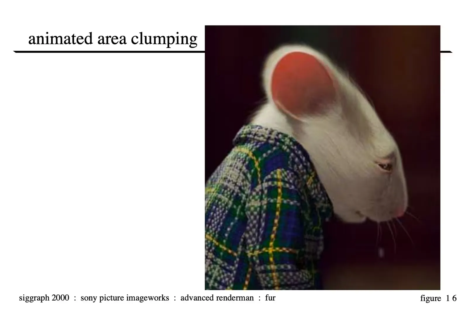 Image Copyright 2000 by Columbia Pictures Industries Inc., All Rights Reserved
Shading
In order to render large amounts of hair quickly and efficiently, the geometric model of each hair is fkept simple. As explained above, a hair is represented by a parametric curve with few control vertices (the default is four). We use the RenderMan RiCurves primitive to render the final hairs. This primitive consists of many small micro-polygons falling along a specified (hair) curve with their normals pointing directly towards the camera (like a 2-dimensional ribbon always oriented towards the camera). In comparison to long tubes, these primitives render extremely efficiently. However, we still need to solve the problem of how to properly shade these primitives as if they were thin hairs.
When using a more conventional lighting model for the fur (essentially a Lambert shading model applied to a very small cylinder) we came across a few complications. First, a diffuse model which integrates the contribution of the light as if the normal pointed in all directions around the cylinder leaves fur dark when oriented towards the light. This may be accurate but does not produce images that are very appealing. In our testing, we felt that the reason that this model didn’t work as well was because a lot of the light that fur receives is a results of the bounce of the light off other fur in the character which could be modeled with some sort of global illumination solution, but would be very expensive. The final (and for us the most significant) reason that we chose to develop a new diffuse lighting model for our fur was that it was not intuitive for a TD to light. Most lighting TD’s have become very good at lighting surfaces and the rules by which those surfaces behave. So, our lighting model was designed to be lit in a similar way that you would light a surface while retaining variation over the length of the fur which is essential to get a high quality look.
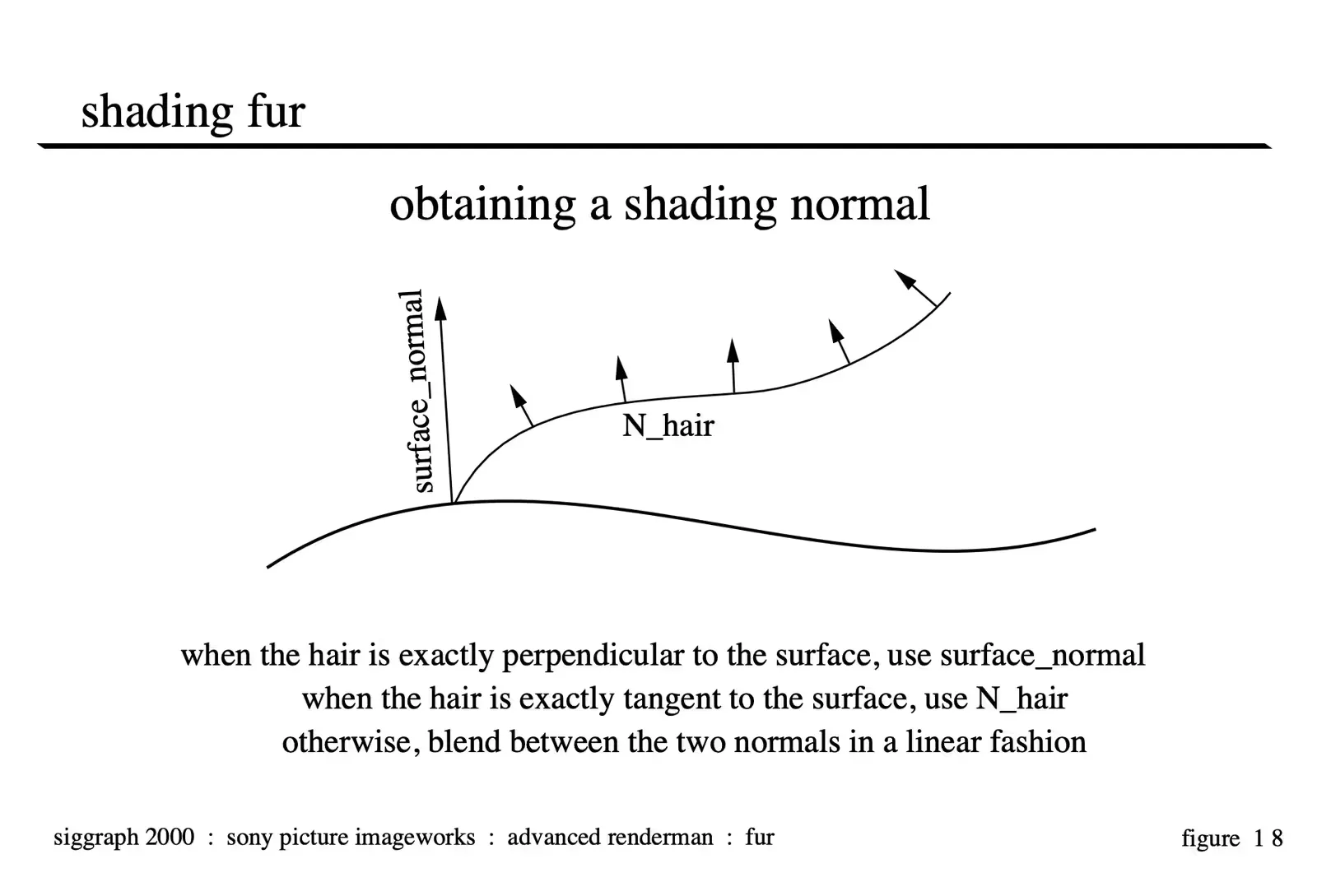
In order to obtain a shading normal at the current point on the hair, we mix the surface normal vector at the base of the hair with the normal vector at the current point on the hair. The amount with which each of these vectors contributes to the mix is based on the angle between the tangent vector at the current point on the hair, and the surface normal vector at the base of the hair. The smaller this angle, the more the surface normal contributes to the shading normal. We then use a Lambertian model to calculate the intensity of the hair at that point using this shading normal. This has the benefit of allowing the user to light the underlying skin surface and then get very predictable results when fur is turned on. It also accounts for shading differences between individual hairs and along the length of each hair.
For the wet fur look, we change two aspects of our regular hair shading process. First, we increase the amount of specular on the fur. Second, we account for clumping in the shading model. Geometrically, as explained earlier, we model fur in clumps to simulate what actually happens when fur gets wet. In the shading model, for each hair, we calculate for each light, what side of the clump the hair is on with respect to the light’s position, and then either darken or brighten the hair based on this. Thus, hairs on the side of a clump facing the light are brighter then hairs on a clump farther from the light.
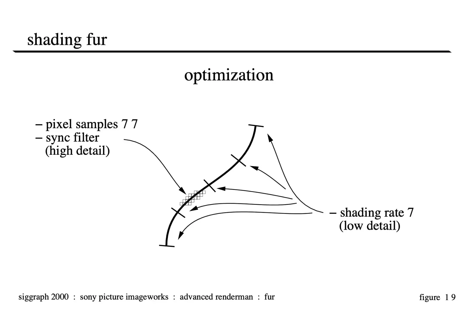
We learned a couple of things through experimentation about optimizing our fur renders. The level of detail requirements along the length of the fur (from one end to another) were very low. Our fur did not consist of many curves or sharp highlights so we could use a very high shading rate and simply allow Renderman to interpolate the shaded values between the samples. This substantially reduced the number of times our shader code needed to be executed and sped up our renders. However, the value for the pixel samples needed to be quite high. We had lots of very thin overlapping curve primitives and without adequate pixel sampling they would alias badly. For most every fur render, our pixel samples needed to be 7 in both directions. We tried different filters as well and found visually that the sinc filter kept more sharpness and did not introduce any objectionable ringing.
Rim Lighting
To give Stuart his characteristic “hero” look it was necessary to have the capability of giving him a nice strong rim light that would wrap in a soft and natural way around the character.
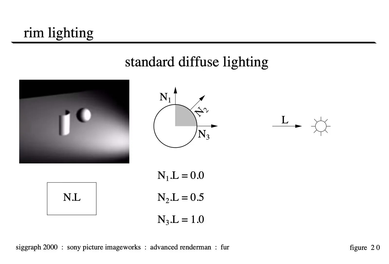 Figure 20 illustrates a standard Lambertian diffuse shading model.
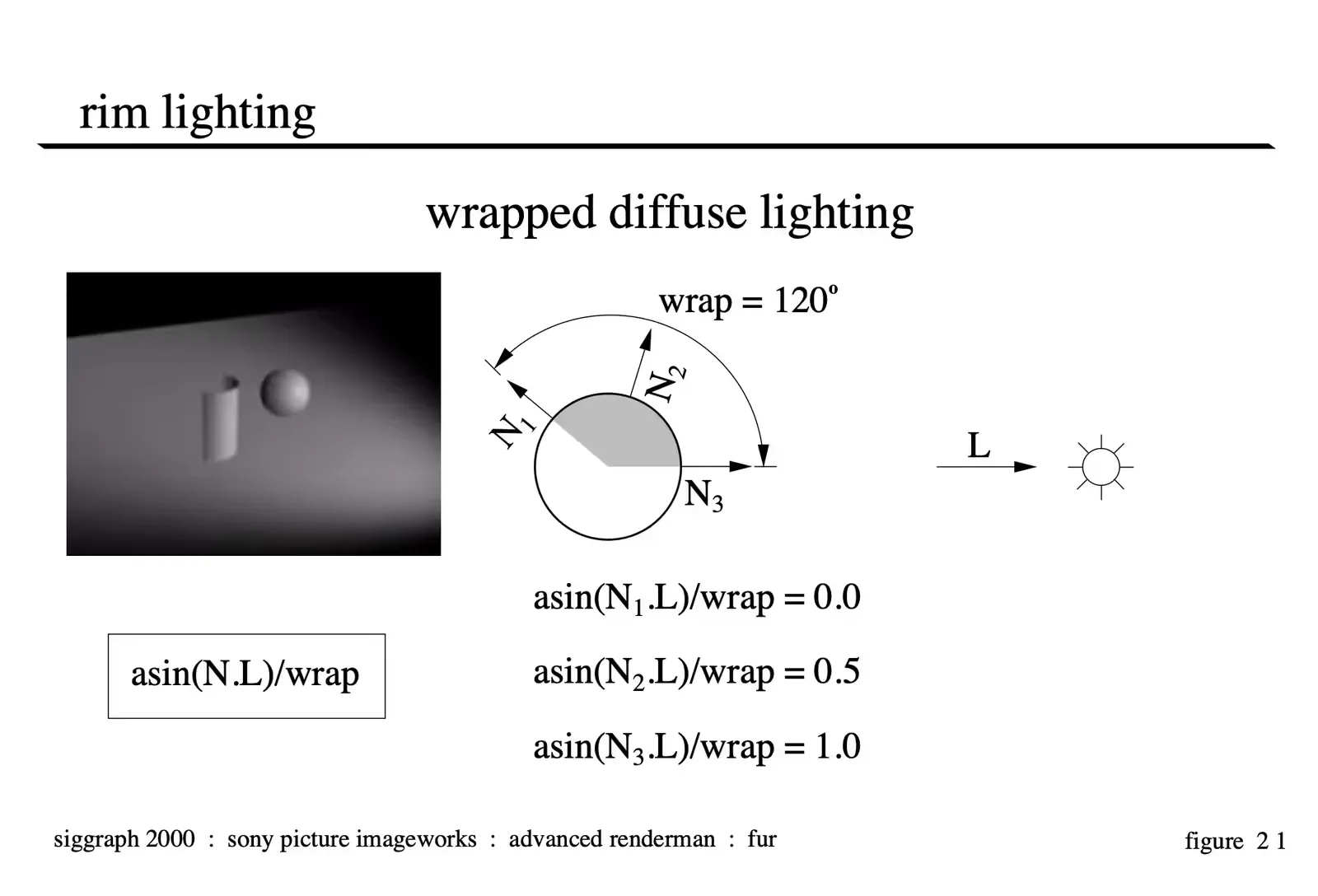
The first step in generating nicely wrapped lighting is to give the light the ability to reach beyond the 90 degree point on the objects. This has the effect of softening the effect of the light on the surface simulating an area light. The controls built into our lights had the ability to specify the end-wrapping-point in terms of degrees where a wrap of 90 degrees corresponded to the standard Lambertian shading model and higher values indicated more wrap. This control was natural for the lighting TD’s to work with and gave predictable results.
For wrapped lights to calculate correctly, the thrid argument to the illuminance statement must be set to at least the same degree as the wrap value for the highest light. Otherwise lights will be culled out from the lighting calculations on the back of the surface and the light will not correctly wrap. In our implemention, the wrap parameter was set in each light and then passed into the shader (using message passing) where we used the customized diffuse calculation to take into account the light wrapping.
As an aside, wrapping the light “more” actually makes the light contribute more energy to the scene. For illustration purposes, the value of the light intensity was halved to generate figure 21.
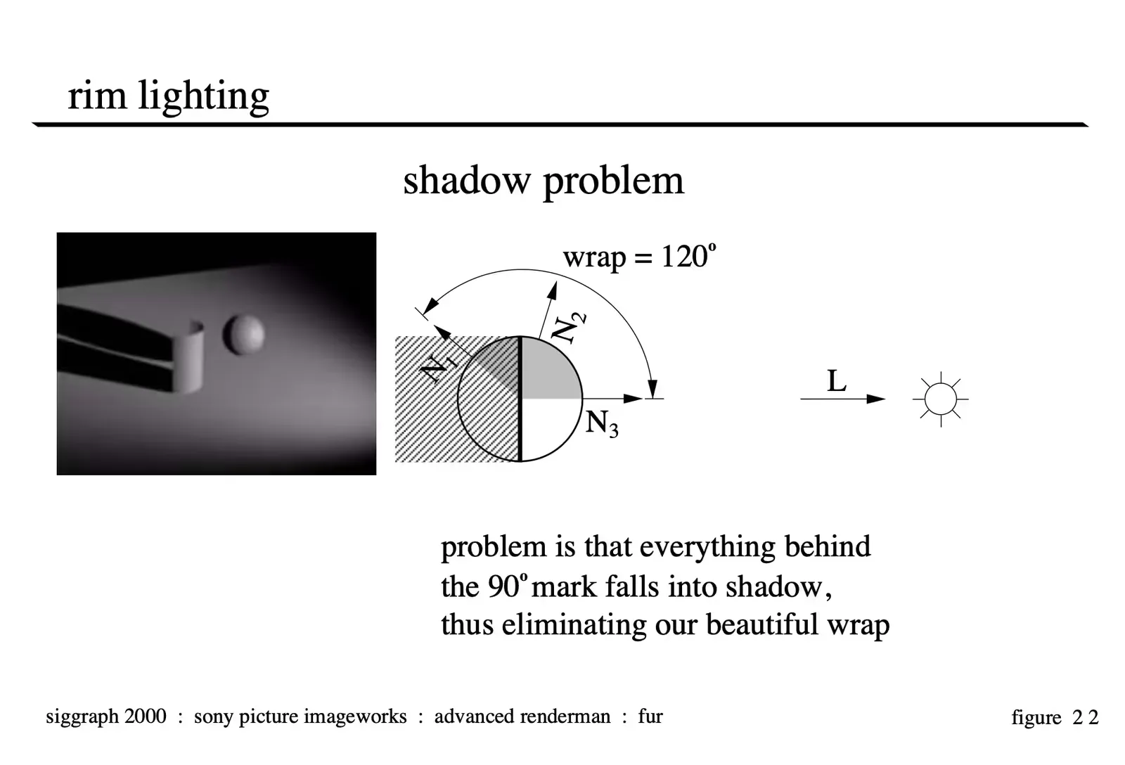
The first problem we encountered when putting these wrapped lights to practical use was with shadow maps. When you have shadow maps for an object, naturally the backside of the object will be made dark because of the shadow call. This makes it impossible to wrap light onto the backside of the object.
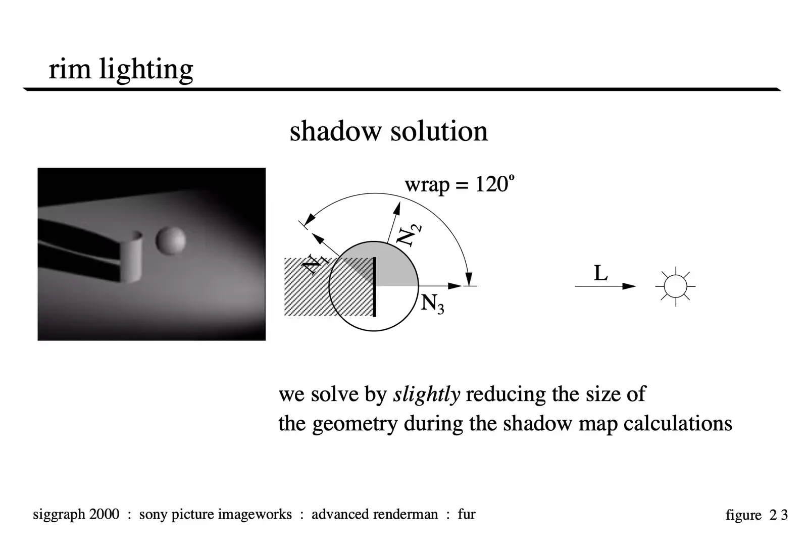
Fortunately Renderman affords a few nice abilities to get around this problem. One way to solve this problem is by reducing the size of your geometry for the shadow map calculations. This way, the object will continue to cast a shadow (albeit a slightly smaller shadow) and the areas that need to catch the wrapped lighting are not occluded by the shadow map.
As a practical matter, shrinking an arbitrary object is not always an easy task. It can be done by displacing the object inwards during the shadow map calculations but this can be very expensive.
In the case of our hair, we wrote opacity controls into the hair shader that were used to drop the opacity of the hair to 0.0 a certain percentage of the way down their length. It is important to note that the surface shader for an object is respected during shadow map calculation and if you set the opacity of a shading point to 0.0, it will not register in the shadow map. The value which is considered “transparent” can be set with the following rib command:
Option "limits" "zthreshold" [0.5 0.5 0.5]Lastly and most simply, you can blur the shadow map when making the “shadow” call. If your requirements are for soft shadows anyway this is probably the best solution of all. It allows for the falloff of the light to “reach around” the object and if there is any occlusion caused by the shadow, it will be occluded softly which will be less objectionable. For Stuart Little, we used a combination of shortening the hair for the shadow map calculations and blurring our shadows to be able to read the appropriate amount of wrap.
 Image Copyright 2000 by Columbia Pictures Industries Inc., All Rights Reserved
Other Tricks: Deformation System
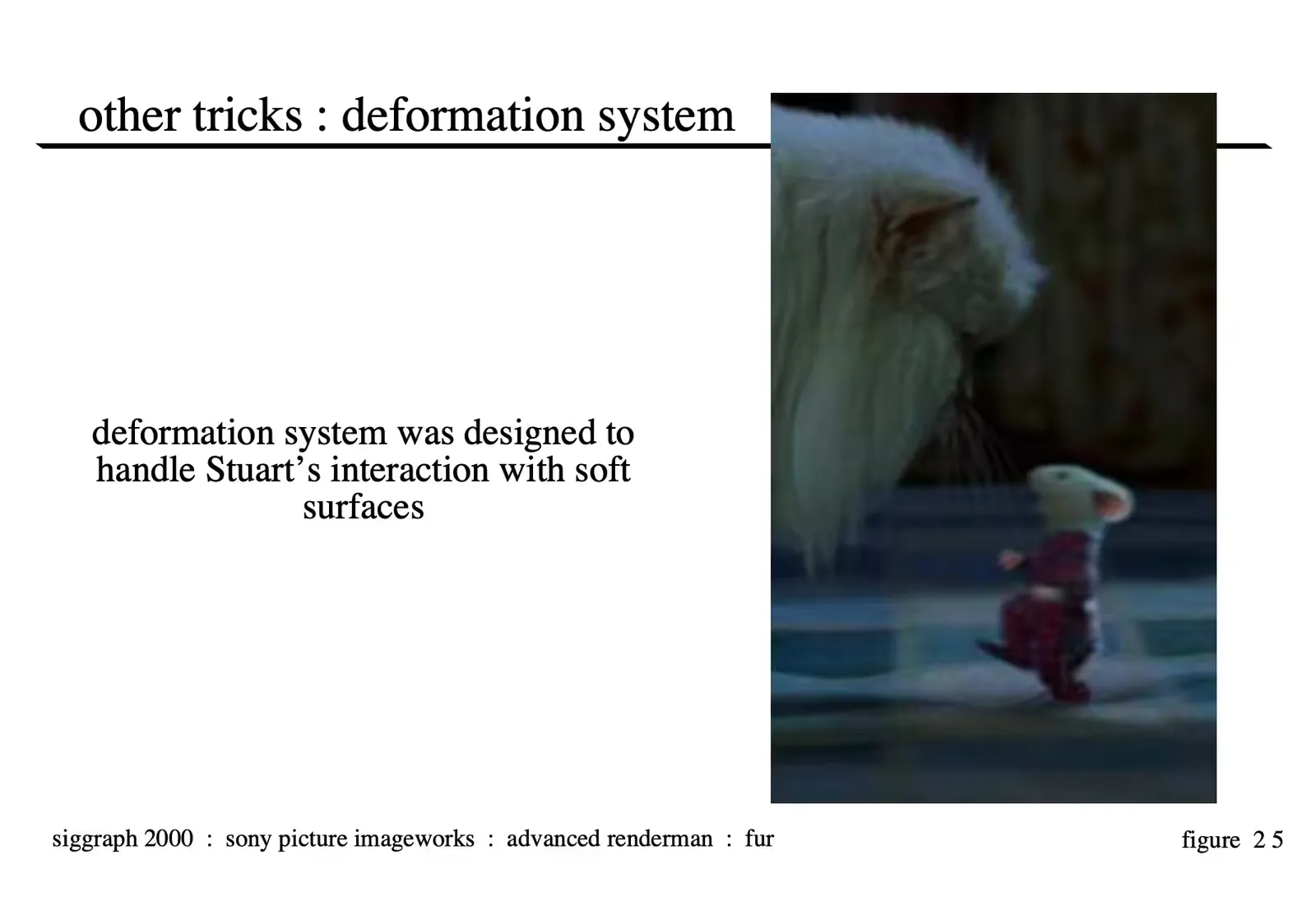 Image Copyright 2000 by Columbia Pictures Industries Inc., All Rights Reserved
Stuart Little called for a number of shots where Stuart needed to interact with a soft environment. For these shots, we developed a system in Renderman to create realistic animation of the surfaces which were generally already in the plate photography. These surfaces needed to be manipulated to appear to be deforming under Stuart’s feet and body.
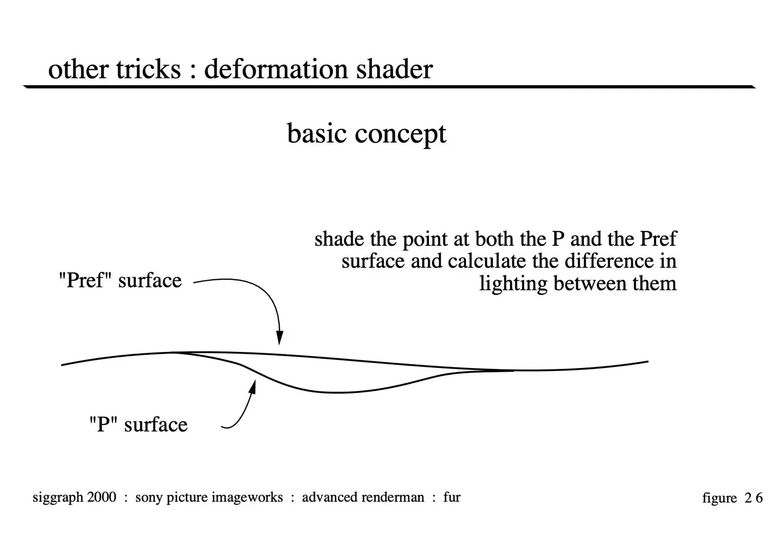
The basic concept behind the system is to create two geometries. The first which represents the surface as it is represented in the plate. If the shot is moving or the surface was animating in the sequence, that surface may be matchmoved frame by frame. For purposes of the discussion of the shader we will refer to this as the “Pref” surface. The second geometry represents the position of the surface when in contact with Stuart. We generate this surface in a variety of ways (one of which will be discussed later), but the basic idea is that the “P” surface is the deformed surface.
To “warp” the plate from the “Pref” to the “P” position is simply a matter of projecting the plate through the scene’s camera onto the “Pref” geometry and then applying that texture to the “P” shading point (see the shader in the appendix for implemenation details).
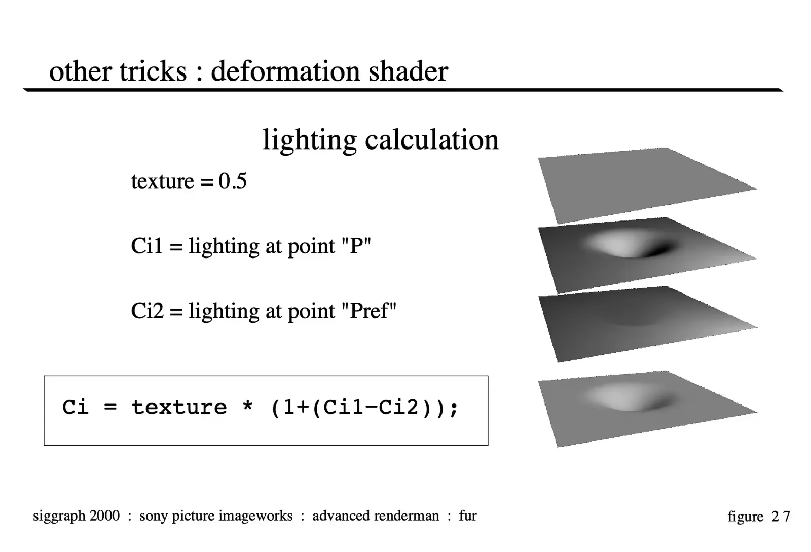
The second thing that needs to be taken into account to make the deformation of the surface appear realistic is the lighting. The approach we take is to measure the lighting intensity on the “P” geometry, measure the lighting on the “Pref” geometry and use the equation illustrated in figure 27 to calculate the brightness change to the plate. This will correctly approximate what would have happened on the set had the same deformation taken place.
This approach generally worked fairly well as long as it wasn’t taken to the extreme. The resolution of the input texture to the system was only the resolution of the film scans of the negative and there is some amount of softening that takes place while projecting and rendering the surface in Renderman. Furthermore, if the stretching is very significant, issues such as the film grain of the plate and other details cannot be ignored. We also found it useful to add a set of color correction parameters that could control how the brightness changes to the plate were specifically applied so that the actual geometry deformation may not need to be re-animated to make a particular part of the deformation appear a little lighter or darker.
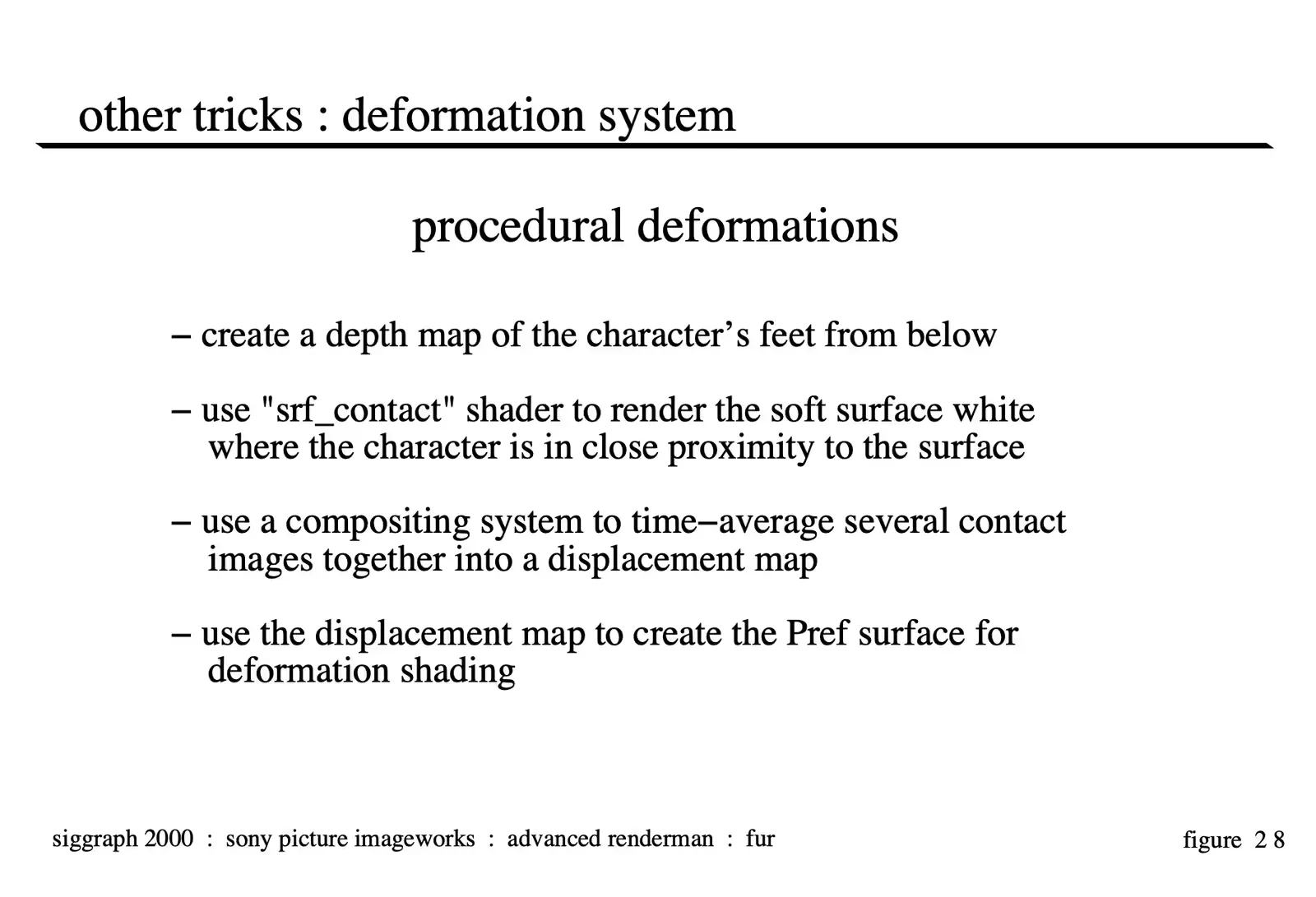
Creating the position of the deformed (or the “P”) object through entirely procedural methods is an interesting task which was developed in Renderman. The first step is to create the “depth map” of the character’s feet (or the part of the body that needs to do the interaction with the surface) from the bottom.
Next, use the depth map as a data file to drive a shader named “srf_contact” which is included as an appendix to these notes. “srf_contact” is applied to the surface to be deformed and will turn to a 1.0 value when the character is within a specified distance from the surface and will gradually fade off as the character gets further away from the surface along the direction vector of the camera used to render the depth file. In our case, this process created a set of images with little white feet that would fade on and off as Stuart’s feet got closer to and further from the surface. This element is named the “contact pass”.
The next step in the process is to sample together several of these images into a new sequence. We used some time filtering techniques by which frame 10 of the sequence would consist of a weighted average of the last 6 frames of the “contact pass”. This enabled a single footprint to leave an impression that would dissapear quickly but not instantaneously in the final deformations. The amount of blur applied to the images can also be animated over time generating footprints that soften as they decompress. This new sequence is generated as a series of “deformation textures”.
The final step is to use those deformation textures as a displacement map to offset the “Pref” surface along the normal or another arbitrary vector to create the “P” surface. Naturally, you can do other interesting things with this displacement map such as add noise or other features to create interesting wrinkles to make the “P” surface appear more natural. But, once the two surfaces are created, the shader described above will calculate the difference between the two surfaces and should yield fairly natural looking results when used in combination with careful lighting.
Other Tricks: textureinfo
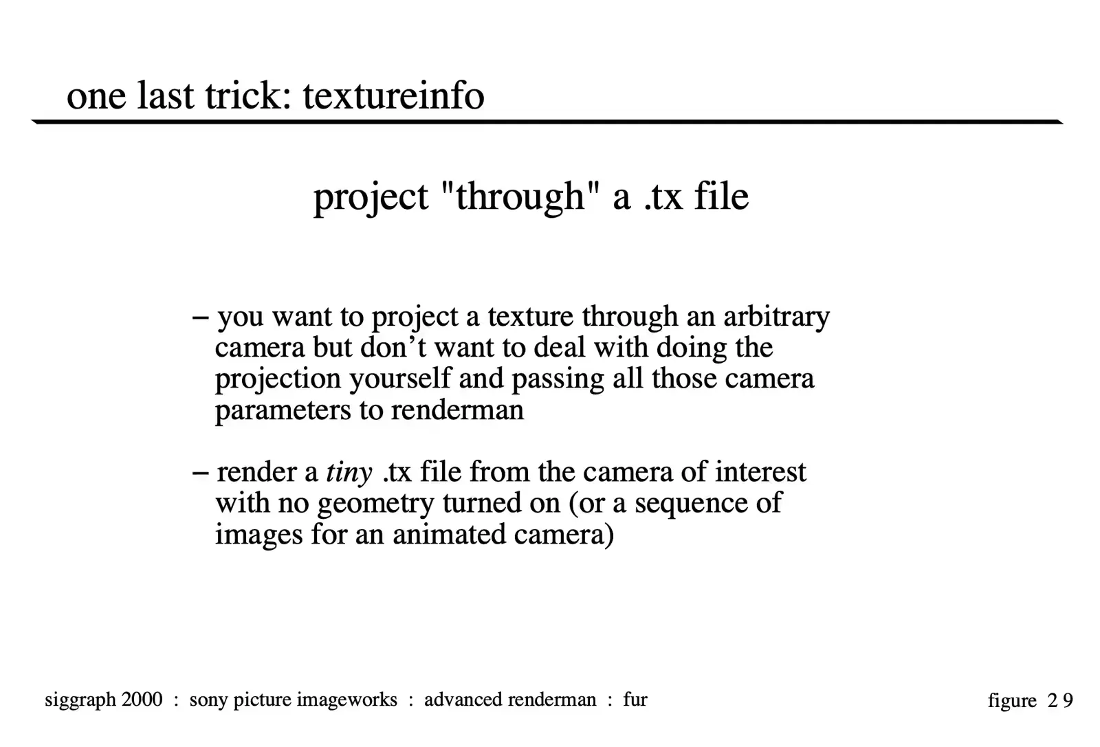
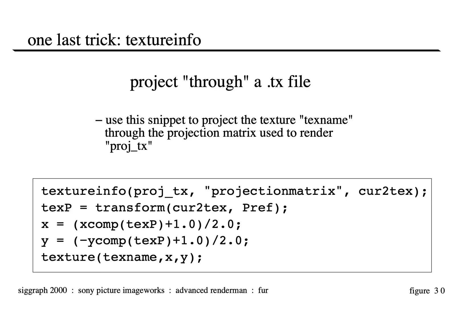
This is simply a handy Renderman technique which has been available since the addition of the “textureinfo” command in version 3.8 of prman. It is mentioned here because it has application in the procedural deformation system—when applying the “deformation textures” back onto the “Pref” geometry if you use this system you can simply project them “through” the “depth file” and they magically always end up in the right position, even with animated cameras. It also has other convenient uses including projecting multiple textures onto a single object for recreating surface detail from multiple still photographs.
Credits
The majority of the development of the fur technology for Stuart Little was performed by Clint Hanson and Armin Bruderlin. Armin also contributed in a large way to these course notes through his paper “A Method to Generate Wet and Broken-up Animal Fur” which was used nearly verbatim to describe the clumping techniques presented herein. Additionally, others who have contributed to the Sony Imageworks hair/fur pipeline are: Alan Davidson, Hiro Miyoshi, Bruce Navsky, Rob Engle, Jay Redd, Amit Agrawal as well as the Imageworks software, digital character, and production groups.
The author also wishes to acknowledge the support of Sony Imageworks for the publication of these notes. It should also be noted that some of the fur methods discussed in this course are techniques for which Sony Imageworks is currently applying for patents.
All figures and illustrations not indicated otherwise are Copyright 2000 by Sony Pictures Imageworks, all rights reserved.
Conclusion
There were several key concepts that made the fur pipeline for Stuart Little a workable solution. Delaying the creation of the largest portion of the dataset until render time was an efficient decision made early in the pipeline design that proved itself in terms of storage and processing time. For the clumping process, the idea of using both a realistic modeling technique combined with shading techniques yielded a strong “wet” fur look. And finally, the decision to use a lighting model which was based more on a TD’s familiarity with lighting surfaces than what would be the most mathmat- ically accurate seemed to give more palatable results in less time, which improved the look of the film.
Shaders
Complete Fur Shader with Clumping and Specular Model
Download srf_fur.sl
/* fur surface shader

   with clumping and specular model

   by Clint Hanson and Armin Bruderlin
*/

color
fnc_diffuselgt (color Cin;       /* Light Colour */
                point Lin;       /* Light Position */
                point Nin;       /* Surface Normal */
    )
{
    color Cout = Cin;
    vector LN, NN;
    float Atten;

    /* normalize the stuff */
    LN = normalize(vector(Lin));
    NN = normalize(vector(Nin));

    /* diffuse calculation */
    Atten = max(0.0,LN.NN);

    Cout *= Atten;

    return (Cout);
}


#define luminance(c) comp(c,0)*0.299 + comp(c,1)*0.587 + comp(c,2)*0.114


surface
srf_fur( /* Hair Shading... */
         float Ka   = 0.0287;
	 float Kd   = 0.77;
	 float Ks   = 1.285;
	 float roughness1  = 0.008;
	 float SPEC1  = 0.01;
	 float roughness2  = 0.016;
	 float SPEC2  = 0.003;
	 float   start_spec = 0.3;
	 float   end_spec = 0.95;
	 float spec_size_fade  = 0.1;
	 float illum_width  = 180;
	 float var_fade_start = 0.005;
	 float var_fade_end = 0.001;
	 float clump_dark_strength = 0.0;

	 /* Hair Color */
	 color rootcolor  = color (.9714, .9714, .9714);
	 color tipcolor = color (.519, .325, .125);
	 color specularcolor  = (color(1) + tipcolor) / 2;
	 color static_ambient  = color (0.057,0.057,0.057);

	 /* Variables Passed from the rib... */
	 uniform float hair_col_var  = 0.0;
	 uniform float hair_length = 0.0;
	 uniform normal surface_normal  = normal 1;
	 varying vector clump_vect  = vector 0;
	 uniform float hair_id   = 0.0; /* Watch Out... Across Patches */

    )
{
    vector T = normalize (dPdv); /* tangent along length of hair */
    vector V = -normalize(I);    /* V is the view vector */
    color Cspec = 0, Cdiff = 0;  /* collect specular & diffuse light */
    float Kspec = Ks;
    vector nL;
    varying normal nSN = normalize( surface_normal );
    vector S = nSN^T;     /* Cross product of the tangent along the hair and surface normal */
    vector N_hair = (T^S); /* N_hair is a normal for the hair oriented "away" from the surface */
    vector norm_hair;
    float  l = clamp(nSN.T,0,1);  /* Dot of surface_normal and T, used for blending */
    float clump_darkening = 1.0;
    float T_Dot_nL = 0;
    float T_Dot_e = 0;
    float Alpha = 0;
    float Beta = 0;
    float Kajiya = 0;
    float darkening = 1.0;
    varying color final_c;

    /* values from light */
    uniform float nonspecular = 0;
    uniform color SpecularColor = 1;

    /* When the hair is exactly perpendicular to the surface, use the
       surface normal, when the hair is exactly tangent to the
       surface, use the hair normal Otherwise, blend between the two
       normals in a linear fashion
    */
    norm_hair = (l * nSN) + ( (1-l) * N_hair);
    norm_hair = normalize(norm_hair);

    /* Make the specular only hit in certain parts of the hair--v is
       along the length of the hair
    */
    Kspec *= min( smoothstep( start_spec, start_spec + spec_size_fade, v),
		  1 - smoothstep( end_spec, end_spec - spec_size_fade, v ) );


    /* Loop over lights, catch highlights as if this was a thin cylinder,

       Specular illumination model from:
       James T. Kajiya and Timothy L.  Kay (1989) "Rendering Fur with Three
       Dimensional Textures", Computer Graphics 23,3, 271-280
    */

    illuminance (P, norm_hair, radians(illum_width)) {
	nL = normalize(L);

	T_Dot_nL = T.nL;
	T_Dot_e = T.V;
	Alpha = acos(T_Dot_nL);
	Beta = acos(T_Dot_e);

	Kajiya = T_Dot_nL * T_Dot_e + sin(Alpha) * sin(Beta);

	/* calculate diffuse component */
	if ( clump_dark_strength > 0.0 ) {
	    clump_darkening = 1 - ( clump_dark_strength *
                                    abs(clamp(nL.normalize(-1*clump_vect), -1, 0)));
	} else {
	    clump_darkening = 1.0;
	}

	/* get light source parameters */
	if ( lightsource("__nonspecular",nonspecular) == 0)
	    nonspecular = 0;
	if ( lightsource("__SpecularColor",SpecularColor) == 0)
	    SpecularColor = color 1;

	Cspec += (1-nonspecular) * SpecularColor * clump_darkening *
	    ((SPEC1*Cl*pow(Kajiya, 1/roughness1)) +
	     (SPEC2*Cl*pow(Kajiya, 1/roughness2)));

	Cdiff += clump_darkening * fnc_diffuselgt(Cl, L, norm_hair);
    }

    darkening = clamp(hair_col_var, 0, 1);

    darkening = (1 - (smoothstep( var_fade_end, var_fade_start,
				  abs(luminance(Kd*Cdiff))) * darkening));

    final_c = mix( rootcolor, tipcolor, v ) * darkening;

    Ci =  ((Ka*ambient() + Kd*Cdiff + static_ambient) * final_c
	   + ((v) * Kspec * Cspec * specularcolor));

    Ci = clamp(Ci, color 0, color 1 );

    Oi = Os;
    Ci = Oi * Ci;
}
Deformation Shader
Download srfdefor.sl
/*
   deformation surface shader

   projects a texture through the camera onto the Pref
   object and deforms it to the P position

   additionally, calculates the changes to shading on the surface
   measured by the change in diffuse lighting from the Pref to P.

   additional contrast and color controls are left as an exersize
   for the user.

   by Rob Bredow and Scott Stokdyk
*/

color
fnc_mydiffuse (color Cl;
	       vector L;
	       normal N)
{
    normal Nn;
    vector Ln;

    Nn = normalize(N);
    Ln = normalize(L);
    return Cl * max(Ln.Nn,0);
}


void
fnc_projectCurrentCamera(point P;
			 output float X, Y;)
{
    point Pndc = transform("NDC", P);

    X = xcomp(Pndc);
    Y = ycomp(Pndc);
}


surface
srf_deformation(
    string texname = "";        /* Texture to project */
    float debug = 0;            /* 0 = deformed lit image
				   1 = texture deformed with no lighting
				   2 = output lighting of the P object
				   3 = output lighting of the Pref object
				*/
    float Kd=1;                 /* Surface Kd for lighting calculations */

    varying point Pref = point "shader" (0,0,0);
    )
{
    float x, y;
    color Ci0, Ci1, Ci2;
    normal N1, N2;
    float illum_width = 180;

    point Porig = Pref;

    fnc_projectCurrentCamera(Pref, x, y);

    if (texname != "") {
	Ci0 = texture(texname, x, y);
    }
    else Ci0 = 0.5;

    /* Calculate shading difference between P and Porig*/

    N = normalize(calculatenormal(P));
    N1 = faceforward(normalize(N),I);
    N = normalize(calculatenormal(Porig));
    N2 = faceforward(normalize(N),I);

    Ci1 = 0.0; Ci2 = 0.0;

    /* These lighting loops can be enhanced to calculate
       specular or reflection maps if needed */

    illuminance(P, N1, radians(illum_width)) {
	Ci1 += Kd * fnc_mydiffuse(Cl,L,N1);
    }

    illuminance(Porig, N2, radians(illum_width)) {
	Ci2 += Kd * fnc_mydiffuse(Cl,L,N2);
    }

    /* Difference in lighting acts as brightness control*/

    Ci = Ci0 * (1+(Ci1-Ci2));
    Oi = 1.0;

    if (debug == 1) {  /* output the texture - no lighting */
	Ci = Ci0;
    } else if (debug == 2) { /* output texture with P's lighting */
	Ci = Ci1;
    } else if (debug == 3) { /* output texture with Pref's lighting */
	Ci = Ci2;
    }
}
Contact “Shadow” Shader
Download srfconta.sl
/*
**
** Render a contact shadow based on depth data derived from a light
** placed onto the surface which catches the contact shadow
**
** by Rob Engle and Jim Berney
*/

surface
srf_contact (
    string shadowname = "";     /* the name of the texture file */
    float samples = 10;         /* how many samples to take per Z lookup */
    float influence = 1.0;      /* world space distance in which effect is visible */
    float gamma = 0.5;          /* controls ramp on of effect over distance */
    float maxdist = 10000;      /* how far is considered infinity */
    )
{
    /* get a matrix which transforms from current space to the
       camera space used when rendering the shadow map */
    uniform matrix matNl;
    textureinfo(shadowname, "viewingmatrix", matNl);

    /* get a matrix which transforms from current space to the
       screen space (-1..1) used when rendering the shadow map */
    uniform matrix matNP;
    textureinfo(shadowname, "projectionmatrix", matNP);

    /* transform the ground plane point into texture coordinates
       needed to look up the point in the shadow map */
    point screenP = transform(matNP, P);
    float ss = (xcomp(screenP) + 1) * 0.5;
    float tt = (1 - ycomp(screenP)) * 0.5;

    if (ss < 0 || ss > 1 || tt < 0 || tt > 1) {
	/* point being shaded is outside the region of the depth map */
	Ci = color(0);
    }
    else {
	/* get the distance from the shadow camera to the closest
	   object as recorded in the shadow map */
	float mapdist = float texture(shadowname, ss, tt, "samples", samples);

	/* transform the point on the ground plane into the shadow
	   camera space in order to get the distance from the shadow
	   camera to the ground plane */
	point cameraP = transform(matNl, P);

	/* the difference between the two distances is used to calculate the
	   contact shadow effect */
	float distance = mapdist - zcomp(cameraP);

	distance = smoothstep(0, 1, distance/influence);
	distance = pow(distance, gamma);

	/* convert into a color (white=shadow) */
	Ci = (1.0-distance);
    }
}
